10 Excel 2013 Advanced Formulas and Functions: Master Data Analysis with Pro-Level Tools

Struggling to evaluate datasets where multiple conditions must align before a result appears? Array formulas in Excel 2013 let you perform complex logic in a single cell—no helper columns required. This is a game-changer for auditors or analysts juggling criteria like "revenue > $10K AND region = 'West' AND quarter = Q3."

To use them, press Ctrl+Shift+Enter after typing your formula (e.g., {=SUM(IF((A2:A100>10000)(B2:B100="West")(C2:C100=3),D2:D100))}). Excel treats it as an array, evaluating every row instantly. The formula returns #VALUE! if entered without the array syntax, so remember the shortcut. For multi-criteria sums or counts, this cuts manual work by 80%.

Perfect for finance teams reconciling budgets or supply chain analysts tracking inventory across regions and time periods. Master this, and you’ll reclaim hours weekly. ✨

Tired of VLOOKUP’s limitations—like rigid column positions or #N/A errors when data shifts? The INDEX-MATCH combo solves these headaches by letting you look up values horizontally or vertically without restructuring your data.

Here’s how it works: INDEX pinpoints the exact cell (e.g., INDEX(A2:A10, 3) grabs the 3rd row), while MATCH finds the row/column number (e.g., MATCH("Apple", B2:B10, 0) returns 2). Combined, they outperform VLOOKUP by handling left-to-right lookups and avoiding errors when columns reorder. For example, merge customer lists from two spreadsheets by matching IDs—no pivot tables required.

Database managers and analysts merging disparate datasets (like sales and inventory tables) will love this pair. It’s also your go-to for dynamic reports where data updates frequently. ⚡

Tired of manually updating reports every time your data changes? Excel 2013’s dynamic array functions like TRANSPOSE and OFFSET let you automate layouts and references without touching a single cell.

Use TRANSPOSE to flip rows into columns (or vice versa) instantly, while OFFSET lets you reference ranges dynamically—ideal for dashboards that pull data from shifting tables. Even INDIRECT lets you pull ranges from cell references, making your spreadsheets adapt to changes automatically. These functions were the backbone of pre-Excel 365 dynamic arrays, and they still handle complex tasks like generating pivot-like summaries without helper columns.

Perfect for accountants managing quarterly reports or operations teams tracking inventory shifts—no manual copy-pasting required. ✨

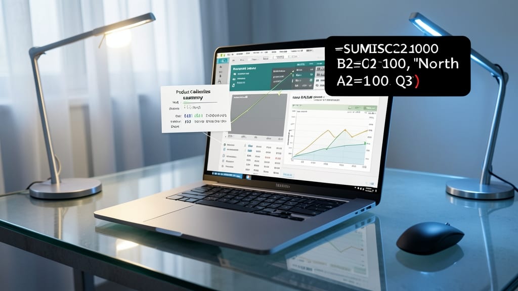
Tired of pivot tables for every financial breakdown? SUMIFS and DSUM let you sum data across multiple criteria in a single formula—no extra steps required. Whether you're tracking sales by region, product category, and quarter, these functions handle the heavy lifting with precision.

SUMIFS (short for "sum if") lets you specify up to 127 conditions (e.g., =SUMIFS(sumrange, criteriarange1, criteria1, criteria_range2, criteria2)). For database-style data, DSUM pulls from structured tables using criteria ranges, making it ideal for large datasets. Both avoid the complexity of helper columns or macros, saving hours on manual calculations.

Financial analysts and operations teams will love these for real-time reporting—no need to rebuild pivot tables every time criteria change. Mastering them cuts down on errors and speeds up decision-making. ✨

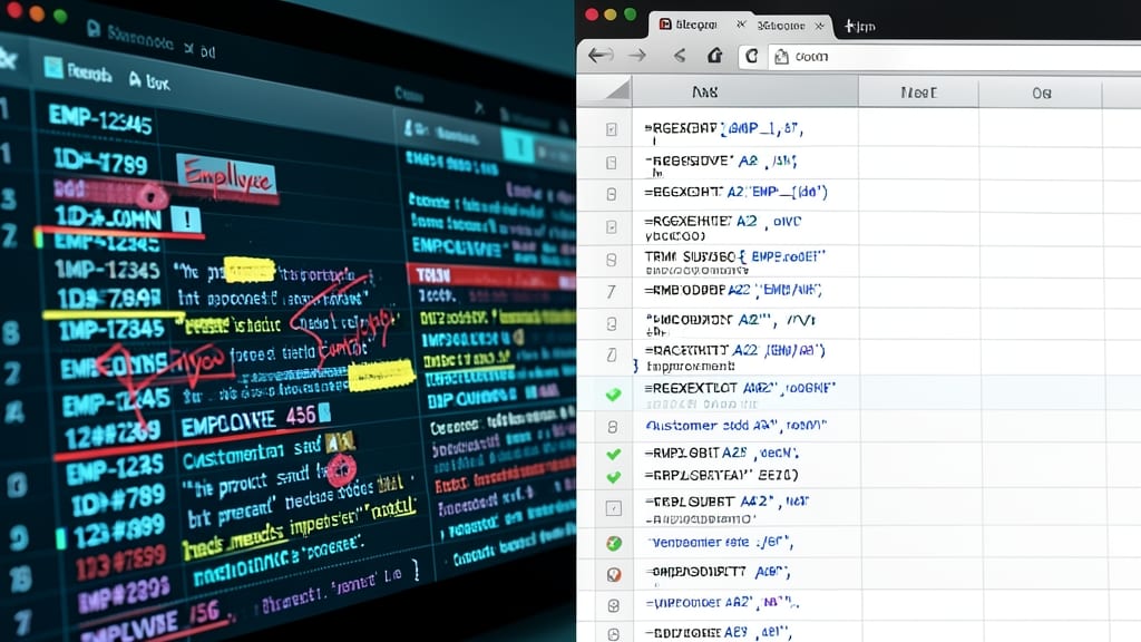
Messy text data—like employee IDs with inconsistent formatting or customer feedback with typos—can derail even the most critical reports. REGEX (regular expressions) and wildcards in Excel 2013 let you extract, clean, or validate text patterns with surgical precision, turning unruly data into structured insights.

Excel’s wildcards (, ?, ~) handle simple tasks like finding partial matches (e.g., Smith*), while REGEX (via the REGEXEXTRACT or REGEXMATCH functions in add-ins like RegexLib) tackles complex patterns. For example, extract email addresses from a column using REGEXEXTRACT(A2, "[A-Za-z0-9._%+-]+@[A-Za-z0-9.-]+\.[A-Za-z]{2,4}"), or validate phone numbers with REGEXMATCH(B2, "^\(\d{3}\) \d{3}-\d{4}$").

HR teams can standardize SSNs or job titles, while marketers can pull product names or sentiment keywords from reviews—all without manual copy-pasting. For Excel 2013, third-party tools like RegexLib bridge the gap since native support is limited. 💡

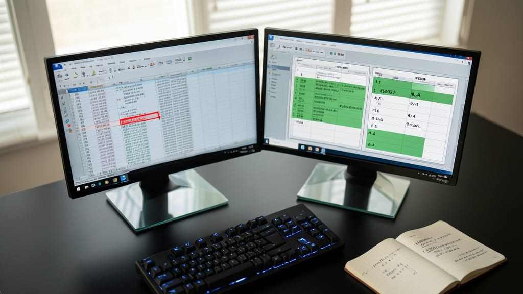
Tired of Excel throwing up #DIV/0! or #N/A errors that break your formulas? IFERROR and ISERROR are your secret weapons for keeping spreadsheets running smoothly—especially in automated systems like inventory tracking where errors can derail entire workflows.

Use IFERROR to return a custom value when a formula fails (e.g., =IFERROR(A1/B1, "Check data")), while ISERROR lets you test for errors first with nested logic like =IF(ISERROR(A1), "Invalid", A1). Both work in Excel 2013 without requiring arrays, making them perfect for real-time data validation in financial models or logistical calculations.

Inventory managers and supply chain analysts will love these for automated stock alerts—no more manual fixes when formulas hit snags. ✨

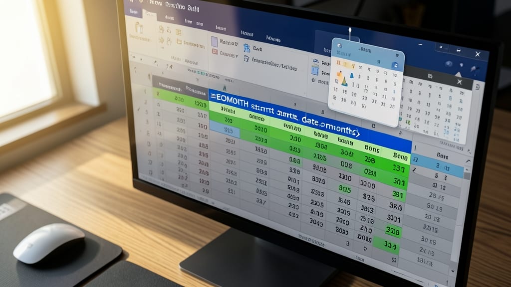
Tired of manually adjusting end-of-month dates in payroll or billing spreadsheets? The EOMONTH function in Excel 2013 automates this with precision, handling leap years and varying month lengths seamlessly.

Simply use =EOMONTH(start_date, months) to return the last day of a month—whether it’s 28, 30, or 31 days. For example, =EOMONTH("1/15/2023", 2) instantly calculates February 28, 2023, even if you’re working with a dataset of thousands of records. Pair it with TODAY() for dynamic calculations, like subscription renewals or project deadlines.

This is a game-changer for HR departments managing payroll cycles or subscription-based businesses automating billing. No more guessing—just reliable, automated date logic. ✨

Tired of repeating the same calculations across workbooks? VBA custom functions let you turn repetitive tasks into reusable code—like a personal library of Excel superpowers. Unlike native functions, these run in the background, accepting inputs and returning results seamlessly, even across multiple files.

With VBA integration, you can create functions like CalculateTaxWithDeductions() or CleanEmailAddresses() that run with a simple formula call (e.g., =CleanEmailAddresses(A2:A100)). The Developer tab in Excel 2013 unlocks the VBA editor, where you write functions in Visual Basic—no prior coding experience required for basic automation. For example, a single custom function can replace dozens of nested IF statements, cutting processing time by 90% for large datasets.

Perfect for accountants automating tax calculations, data analysts cleaning messy datasets, or developers standardizing workflows across teams. Once built, your functions become part of Excel’s formula library, ready to use anywhere. ✨

Turn raw historical data into actionable predictions with FORECAST and TREND—Excel 2013’s secret weapons for statistical analysis. These functions let you project future values based on past trends, whether you’re forecasting quarterly sales, predicting equipment wear, or planning inventory levels.

The FORECAST function uses linear regression to estimate a future value based on existing data points, while TREND extends this by returning an entire trendline. Both support up to 255 data points and work seamlessly with charts for visual validation. For example, input monthly sales data to predict next quarter’s revenue with just three arguments—no complex add-ins required.

Operations managers and financial analysts will find these tools indispensable for data-driven decision-making, while marketers can use them to model campaign performance. ⚡

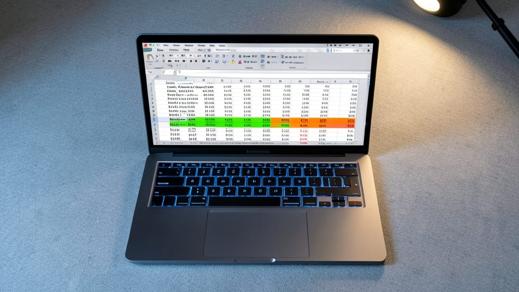
Tired of drowning in raw numbers during presentations? Advanced Conditional Formatting Rules in Excel 2013 let you highlight data patterns automatically—no manual color-coding required. With rules like "highlight cells where sales exceed $10K and growth is >10%," you turn static tables into visual stories that executives grasp instantly.

Excel 2013 supports up to three conditions per rule (e.g., date ranges + performance metrics), plus color scales and icon sets to show trends at a glance. Combine this with data bars for quick comparisons, and your dashboards become self-explanatory. The best part? Rules update dynamically—change your data, and the formatting adjusts automatically.

Perfect for finance teams presenting quarterly reports or operations managers tracking KPIs. Skip the PowerPoint slides—let your data speak for itself. ✨